Bayesian initial condition inversion in an advection-diffusion problem
In this example we tackle the problem of quantifying the uncertainty in the solution of an inverse problem governed by a parabolic PDE via the Bayesian inference framework. The underlying PDE is a time-dependent advection-diffusion equation in which we seek to infer an unknown initial condition from spatio-temporal point measurements.
The Bayesian inverse problem:
Following the Bayesian framework, we utilize a Gaussian prior measure , with where is an elliptic differential operator as described in the PoissonBayesian example, and use an additive Gaussian noise model. Therefore, the solution of the Bayesian inverse problem is the posterior measure, with and .
- The posterior mean is characterized as the minimizer of
which can also be interpreted as the regularized functional to be minimized in deterministic inversion. The observation operator extracts the values of the forward solution on a set of locations at times .
- The posterior covariance is the inverse of the Hessian of , i.e.,
The forward problem:
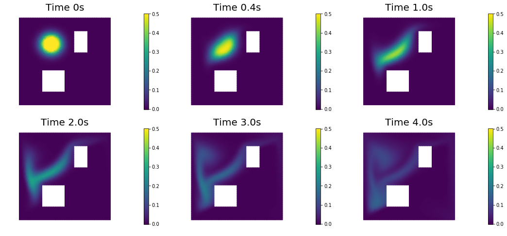
The parameter-to-observable map maps an initial condition to pointwise spatiotemporal observations of the concentration field through solution of the advection-diffusion equation given by
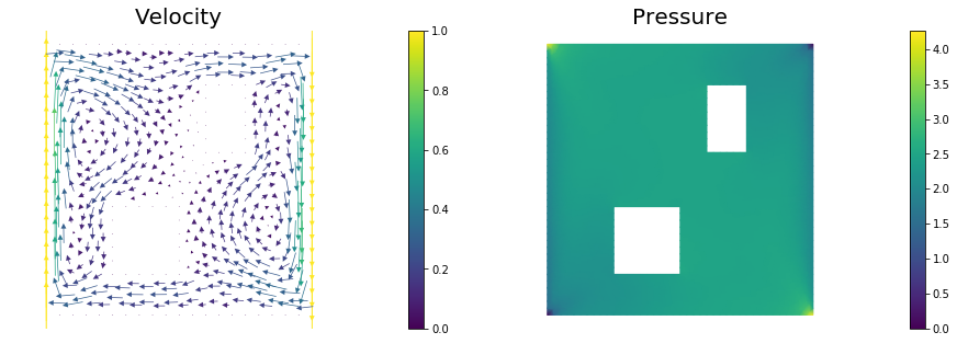
Here, () is a bounded domain, is the diffusion coefficient and is the final time. The velocity field is computed by solving the following steady-state Navier-Stokes equation with the side walls driving the flow:
Here, is pressure, is the Reynolds number. The Dirichlet boundary data is given by on the left wall of the domain, on the right wall, and everywhere else.
The adjoint problem:
The adjoint problem is a final value problem, since is specified at rather than at . Thus, it is solved backwards in time, which amounts to the solution of the advection-diffusion equation
Then, the adjoint of the parameter to observable map is defined by setting
1. Load modules
from __future__ import absolute_import, division, print_function

import dolfin as dl
import math
import numpy as np
import matplotlib.pyplot as plt
%matplotlib inline
import sys
import os
sys.path.append( os.environ.get('HIPPYLIB_BASE_DIR', "../") )
from hippylib import *
sys.path.append( os.environ.get('HIPPYLIB_BASE_DIR', "..") + "/applications/ad_diff/" )
from model_ad_diff import TimeDependentAD, SpaceTimePointwiseStateObservation

import logging
logging.getLogger('FFC').setLevel(logging.WARNING)
logging.getLogger('UFL').setLevel(logging.WARNING)
dl.set_log_active(False)
2. Construct the velocity field
def v_boundary(x,on_boundary):
    return on_boundary

def q_boundary(x,on_boundary):
    return x[0] < dl.DOLFIN_EPS and x[1] < dl.DOLFIN_EPS

def computeVelocityField(mesh):
    Xh = dl.VectorFunctionSpace(mesh,'Lagrange', 2)
    Wh = dl.FunctionSpace(mesh, 'Lagrange', 1)
    if dlversion() <= (1,6,0):
        XW = dl.MixedFunctionSpace([Xh, Wh])
    else:
        mixed_element = dl.MixedElement([Xh.ufl_element(), Wh.ufl_element()])
        XW = dl.FunctionSpace(mesh, mixed_element)

    Re = 1e2

    g = dl.Expression(('0.0','(x[0] < 1e-14) - (x[0] > 1 - 1e-14)'), degree=1)
    bc1 = dl.DirichletBC(XW.sub(0), g, v_boundary)
    bc2 = dl.DirichletBC(XW.sub(1), dl.Constant(0), q_boundary, 'pointwise')
    bcs = [bc1, bc2]

    vq = dl.Function(XW)
    (v,q) = dl.split(vq)
    (v_test, q_test) = dl.TestFunctions (XW)

    def strain(v):
        return dl.sym(dl.nabla_grad(v))

    F = ( (2./Re)*dl.inner(strain(v),strain(v_test))+ dl.inner (dl.nabla_grad(v)*v, v_test)
           - (q * dl.div(v_test)) + ( dl.div(v) * q_test) ) * dl.dx

    dl.solve(F == 0, vq, bcs, solver_parameters={"newton_solver":
                                         {"relative_tolerance":1e-4, "maximum_iterations":100}})

    plt.figure(figsize=(15,5))
    vh = dl.project(v,Xh)
    qh = dl.project(q,Wh)
    nb.plot(nb.coarsen_v(vh), subplot_loc=121,mytitle="Velocity")
    nb.plot(qh, subplot_loc=122,mytitle="Pressure")
    plt.show()

    return v
3. Set up the mesh and finite element spaces
mesh = dl.refine( dl.Mesh("ad_20.xml") )
wind_velocity = computeVelocityField(mesh)
Vh = dl.FunctionSpace(mesh, "Lagrange", 1)
print( "Number of dofs: {0}".format( Vh.dim() ) )
Number of dofs: 2023
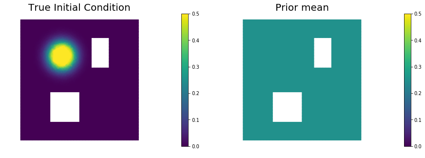
4. Set up model (prior, true/proposed initial condition)
ic_expr = dl.Expression('min(0.5,exp(-100*(pow(x[0]-0.35,2) +  pow(x[1]-0.7,2))))', element=Vh.ufl_element())
true_initial_condition = dl.interpolate(ic_expr, Vh).vector()


gamma = 1.
delta = 8.
prior = BiLaplacianPrior(Vh, gamma, delta, robin_bc=True)
print( "Prior regularization: (delta - gamma*Laplacian)^order: delta={0}, gamma={1}, order={2}".format(delta, gamma,2) )
prior.mean = dl.interpolate(dl.Constant(0.25), Vh).vector()

t_init         = 0.
t_final        = 4.
t_1            = 1.
dt             = .1
observation_dt = .2

simulation_times = np.arange(t_init, t_final+.5*dt, dt)
observation_times = np.arange(t_1, t_final+.5*dt, observation_dt)

targets = np.loadtxt('targets.txt')
print ("Number of observation points: {0}".format(targets.shape[0]) )
misfit = SpaceTimePointwiseStateObservation(Vh, observation_times, targets)

problem = TimeDependentAD(mesh, [Vh,Vh,Vh], prior, misfit, simulation_times, wind_velocity, True)

objs = [dl.Function(Vh,true_initial_condition),
        dl.Function(Vh,prior.mean)]
mytitles = ["True Initial Condition", "Prior mean"]
nb.multi1_plot(objs, mytitles)
plt.show()
Prior regularization: (delta - gamma*Laplacian)^order: delta=8.0, gamma=1.0, order=2
Number of observation points: 80
5. Generate the synthetic observations
rel_noise = 0.01
utrue = problem.generate_vector(STATE)
x = [utrue, true_initial_condition, None]
problem.solveFwd(x[STATE], x, 1e-9)
misfit.observe(x, misfit.d)
MAX = misfit.d.norm("linf", "linf")
noise_std_dev = rel_noise * MAX
parRandom.normal_perturb(noise_std_dev,misfit.d)
misfit.noise_variance = noise_std_dev*noise_std_dev

nb.show_solution(Vh, true_initial_condition, utrue, "Solution")
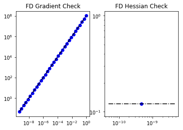
6. Test the gradient and the Hessian of the cost (negative log posterior)
m0 = true_initial_condition.copy()
_ = modelVerify(problem, m0, 1e-12, is_quadratic=True)
(yy, H xx) - (xx, H yy) = -1.174447494183385e-13
7. Evaluate the gradient
[u,m,p] = problem.generate_vector()
problem.solveFwd(u, [u,m,p], 1e-12)
problem.solveAdj(p, [u,m,p], 1e-12)
mg = problem.generate_vector(PARAMETER)
grad_norm = problem.evalGradientParameter([u,m,p], mg)

print( "(g,g) = ", grad_norm)
(g,g) = 2395071437584061.5
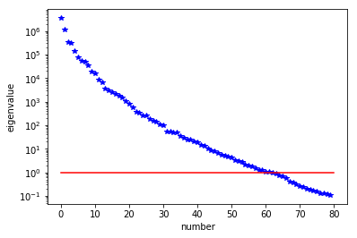
8. The Gaussian posterior
H = ReducedHessian(problem, 1e-12, misfit_only=True)
k = 80
p = 20
print( "Single Pass Algorithm. Requested eigenvectors: {0}; Oversampling {1}.".format(k,p) )
Omega = MultiVector(x[PARAMETER], k+p)
parRandom.normal(1., Omega)
lmbda, V = singlePassG(H, prior.R, prior.Rsolver, Omega, k)
posterior = GaussianLRPosterior( prior, lmbda, V )
plt.plot(range(0,k), lmbda, 'b*', range(0,k+1), np.ones(k+1), '-r')
plt.yscale('log')
plt.xlabel('number')
plt.ylabel('eigenvalue')
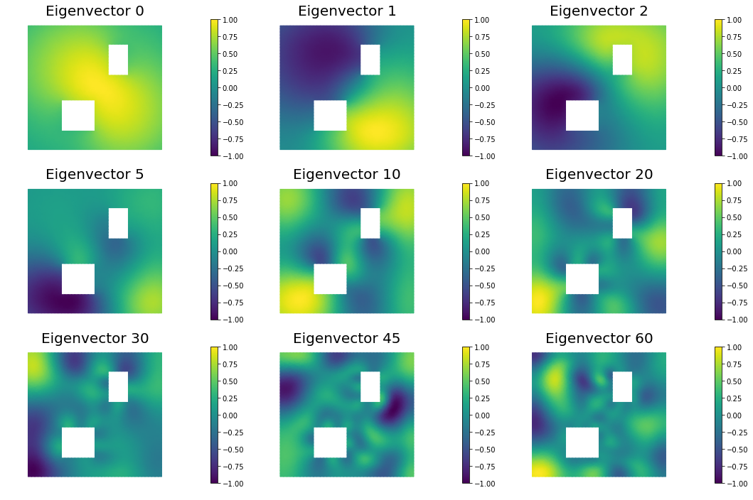
nb.plot_eigenvectors(Vh, V, mytitle="Eigenvector", which=[0,1,2,5,10,20,30,45,60])
Single Pass Algorithm. Requested eigenvectors: 80; Oversampling 20.
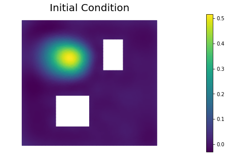
9. Compute the MAP point
H.misfit_only = False
solver = CGSolverSteihaug()
solver.set_operator(H)
solver.set_preconditioner( posterior.Hlr )
solver.parameters["print_level"] = 1
solver.parameters["rel_tolerance"] = 1e-6
solver.solve(m, -mg)
problem.solveFwd(u, [u,m,p], 1e-12)
total_cost, reg_cost, misfit_cost = problem.cost([u,m,p])
print( "Total cost {0:5g}; Reg Cost {1:5g}; Misfit {2:5g}".format(total_cost, reg_cost, misfit_cost) )
posterior.mean = m
plt.figure(figsize=(7.5,5))
nb.plot(dl.Function(Vh, m), mytitle="Initial Condition")
plt.show()
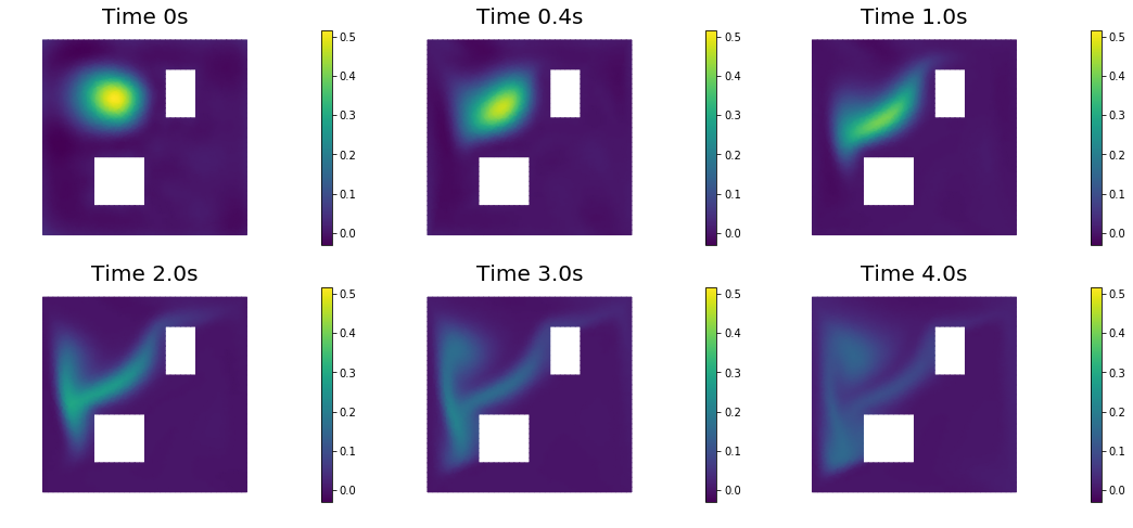
nb.show_solution(Vh, m, u, "Solution")
 Iterartion :  0  (B r, r) =  1225123.9338492027
 Iteration :  1  (B r, r) =  74.94198007028052
 Iteration :  2  (B r, r) =  0.4132940000407347
 Iteration :  3  (B r, r) =  0.005765443940190191
 Iteration :  4  (B r, r) =  2.243708962553132e-05
 Iteration :  5  (B r, r) =  1.4026897765563288e-07
Relative/Absolute residual less than tol
Converged in  5  iterations with final norm  0.0003745250027109444
Total cost 782.818; Reg Cost 153.671; Misfit 629.147
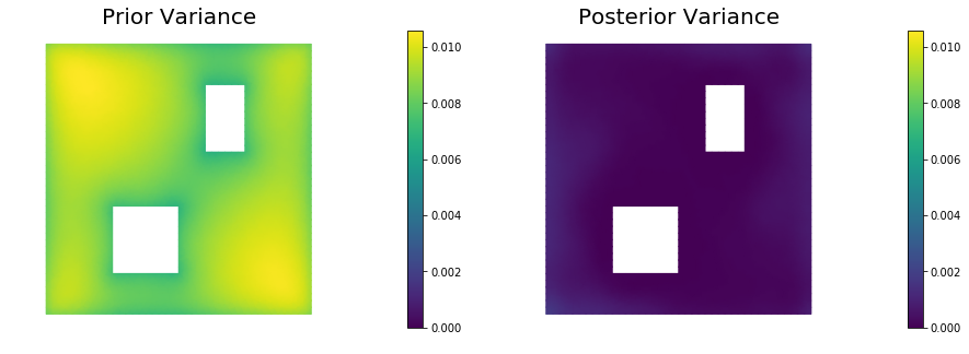
10. Prior and posterior pointwise variance fields
compute_trace = True
if compute_trace:
    post_tr, prior_tr, corr_tr = posterior.trace(method="Randomized", r=300)
    print( "Posterior trace {0:5g}; Prior trace {1:5g}; Correction trace {2:5g}".format(post_tr, prior_tr, corr_tr) )
post_pw_variance, pr_pw_variance, corr_pw_variance = posterior.pointwise_variance(method="Randomized", r=300)

objs = [dl.Function(Vh, pr_pw_variance),
        dl.Function(Vh, post_pw_variance)]
mytitles = ["Prior Variance", "Posterior Variance"]
nb.multi1_plot(objs, mytitles, logscale=False)
plt.show()
Posterior trace 0.000269147; Prior trace 0.00809706; Correction trace 0.00782792
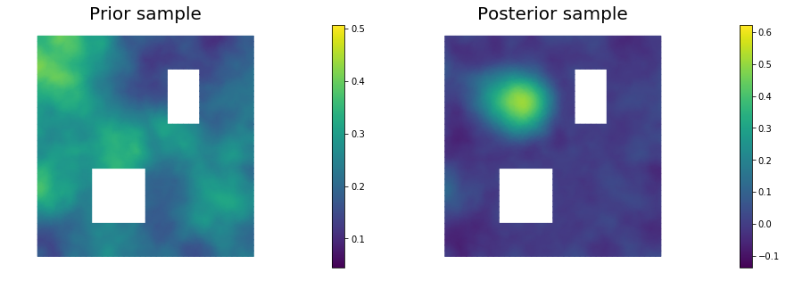
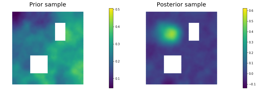
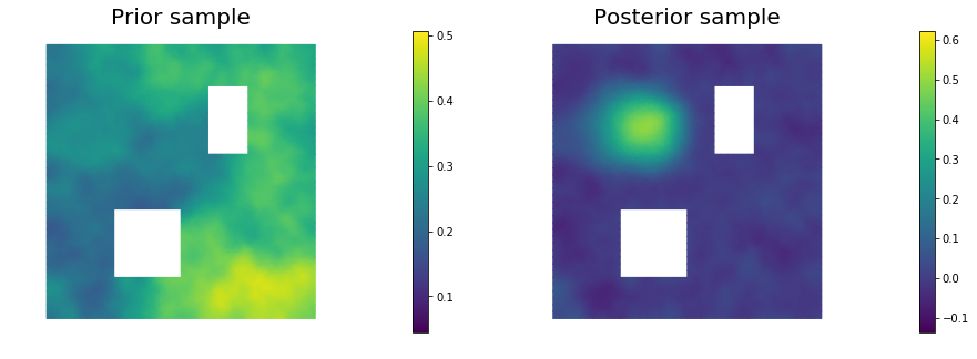
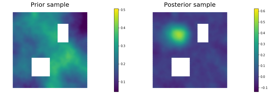
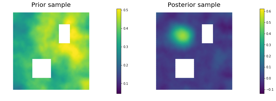
11. Draw samples from the prior and posterior distributions
nsamples = 5
noise = dl.Vector()
posterior.init_vector(noise,"noise")
s_prior = dl.Function(Vh, name="sample_prior")
s_post = dl.Function(Vh, name="sample_post")

pr_max =  2.5*math.sqrt( pr_pw_variance.max() ) + prior.mean.max()
pr_min = -2.5*math.sqrt( pr_pw_variance.min() ) + prior.mean.min()
ps_max =  2.5*math.sqrt( post_pw_variance.max() ) + posterior.mean.max()
ps_min = -2.5*math.sqrt( post_pw_variance.max() ) + posterior.mean.min()

for i in range(nsamples):
    parRandom.normal(1., noise)
    posterior.sample(noise, s_prior.vector(), s_post.vector())
    plt.figure(figsize=(15,5))
    nb.plot(s_prior, subplot_loc=121,mytitle="Prior sample", vmin=pr_min, vmax=pr_max)
    nb.plot(s_post, subplot_loc=122,mytitle="Posterior sample", vmin=ps_min, vmax=ps_max)
    plt.show()
Copyright (c) 2016-2018, The University of Texas at Austin & University of California, Merced.
All Rights reserved.
See file COPYRIGHT for details.
This file is part of the hIPPYlib library. For more information and source code availability see https://hippylib.github.io.
hIPPYlib is free software; you can redistribute it and/or modify it under the terms of the GNU General Public License (as published by the Free Software Foundation) version 2.0 dated June 1991.