FEniCS101 Tutorial
In this tutorial we consider the boundary value problem (BVP)
where , and and are the union of the left and right, and top and bottom boundaries of , respectively.
Here
The exact solution is
Weak formulation
Let us define the Hilbert spaces as
To obtain the weak formulation, we multiply the PDE by an arbitrary function and integrate over the domain leading to
Then, integration by parts the non-conforming term gives
Finally by recalling that on and that on , we find the weak formulation:
Find * such that*
1. Load modules
To start we load the following modules:
-
dolfin: the python/C++ interface to FEniCS
-
math: the python module for mathematical functions
-
numpy: a python package for linear algebra
-
matplotlib: a python package used for plotting the results
from __future__ import absolute_import, division, print_function

from dolfin import *

import math
import numpy as np
import logging

import matplotlib.pyplot as plt
%matplotlib inline
import nb

logging.getLogger('FFC').setLevel(logging.WARNING)
logging.getLogger('UFL').setLevel(logging.WARNING)
set_log_active(False)
2. Define the mesh and the finite element space
We construct a triangulation (mesh) of the computational domain with n elements in each direction.
On the mesh , we then define the finite element space consisting of globally continuous piecewise polinomials functions. The degree variable defines the polinomial degree.
n = 16
degree = 1
mesh = UnitSquareMesh(n, n)
nb.plot(mesh)

Vh  = FunctionSpace(mesh, 'Lagrange', degree)
print("dim(Vh) = ", Vh.dim())
dim(Vh) = 289

3. Define boundary labels
To partition the boundary of in the subdomains , , , we assign a unique label boundary_parts to each of part of .
class TopBoundary(SubDomain):
    def inside(self, x, on_boundary):
        return on_boundary and abs(x[1] - 1) < DOLFIN_EPS

class BottomBoundary(SubDomain):
    def inside(self, x, on_boundary):
        return on_boundary and abs(x[1]) < DOLFIN_EPS

class LeftBoundary(SubDomain):
    def inside(self, x, on_boundary):
        return on_boundary and abs(x[0]) < DOLFIN_EPS

class RightBoundary(SubDomain):
    def inside(self, x, on_boundary):
        return on_boundary and abs(x[0] - 1) < DOLFIN_EPS

boundary_parts = FacetFunction("size_t", mesh)
boundary_parts.set_all(0)

Gamma_top = TopBoundary()
Gamma_top.mark(boundary_parts, 1)
Gamma_bottom = BottomBoundary()
Gamma_bottom.mark(boundary_parts, 2)
Gamma_left = LeftBoundary()
Gamma_left.mark(boundary_parts, 3)
Gamma_right = RightBoundary()
Gamma_right.mark(boundary_parts, 4)
4. Define the coefficients of the PDE and the boundary conditions
We first define the coefficients of the PDE using the Constant and Expression classes. Constant is used to define coefficients that do not depend on the space coordinates, Expression is used to define coefficients that are a known function of the space coordinates x[0] (x-axis direction) and x[1] (y-axis direction).
In the finite element method community, Dirichlet boundary conditions are also known as essential boundary conditions since they are imposed directly in the definition of the finite element space. In FEniCS, we use the class DirichletBC to indicate this type of condition.
On the other hand, Newman boundary conditions are also known as natural boundary conditions since they are weakly imposed as boundary integrals in the variational formulation (weak form). In FEniCS, we create a new boundary measure ds[i] to integrate over the portion of the boundary marked with label i.
u_L = Constant(0.)
u_R = Constant(0.)

sigma_bottom = Expression('-(pi/2.0)*sin(2*pi*x[0])', degree=5)
sigma_top    = Constant(0.)

f = Expression('(4.0*pi*pi+pi*pi/4.0)*(sin(2*pi*x[0])*sin((pi/2.0)*x[1]))', degree=5)

bcs = [DirichletBC(Vh, u_L, boundary_parts, 3),
       DirichletBC(Vh, u_R, boundary_parts, 4)]

ds = Measure("ds", subdomain_data=boundary_parts)
5. Define and solve the variational problem
We also define two special types of functions: the TrialFunction u and the TestFunction v. These special types of function are used by FEniCS to generate the finite element vectors and matrices which stem from the weak formulation of the PDE.
More specifically, by denoting by the finite element basis for the space , a function can be written as where represents the coefficients in the finite element expansion of .
We then define
-
the bilinear form ;
-
the linear form .
We can then solve the variational problem
Find such that
using directly the built-in solve method in FEniCS.
NOTE: As an alternative one can also assemble the finite element matrix and the right hand side that stems from the discretization of and , and then solve the linear system where
-
is the vector collecting the coefficient of the finite element expasion of ,
-
the entries of the matrix A are such that ,
-
the entries of the right hand side b are such that .
u = TrialFunction(Vh)
v = TestFunction(Vh)
a = inner(nabla_grad(u), nabla_grad(v))*dx
L = f*v*dx + sigma_top*v*ds(1) + sigma_bottom*v*ds(2)

uh = Function(Vh)

#solve(a == L, uh, bcs=bcs)
A, b = assemble_system(a,L, bcs=bcs)
solve(A, uh.vector(), b, "cg")

nb.plot(uh)
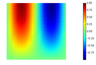
6. Compute the discretization error
For this problem, the exact solution is known. We can therefore compute the following norms of the discretization error (i.e. the of the difference between the finite element solution and the exact solution ) and
u_e = Expression('sin(2*pi*x[0])*sin((pi/2.0)*x[1])', degree=5)
grad_u_e = Expression( ('2*pi*cos(2*pi*x[0])*sin((pi/2.0)*x[1])', 'pi/2.0*sin(2*pi*x[0])*cos((pi/2.0)*x[1])'), degree=5)

err_L2 = sqrt( assemble( (uh-u_e)**2*dx ) )
err_grad = sqrt( assemble( inner(nabla_grad(uh) - grad_u_e, nabla_grad(uh) - grad_u_e)*dx ) )
err_H1 = sqrt( err_L2**2 + err_grad**2)

print("|| u_h - u_e ||_L2 = ", err_L2)
print("|| u_h - u_e ||_H1 = ", err_H1)
|| u_h - u_e ||_L2 =  0.00880525372208
|| u_h - u_e ||_H1 =  0.396718952514
7. Convergence of the finite element method
We now verify numerically a well-known convergence result for the finite element method.
Let denote with the polynomial degree of the finite element space, and assume that the solution is at least in . Then we have
In the code below, the function compute(n, degree) solves the PDE using a mesh with n elements in each direction and finite element spaces of polinomial order degree.
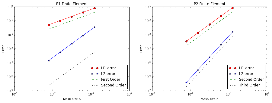
The figure below shows the discretization errors in the and as a function of the mesh size () for piecewise linear (P1, ) and piecewise quadratic (P2, ) finite elements. We observe that numerical results are consistent with the finite element convergence theory. In particular:
-
for piecewise linear finite element P1 we observe first order convergence in the -norm and second order convergence in the -norm;
-
for piecewise quadratic finite element P2 we observe second order convergence in the -norm and third order convergence in the -norm.
def compute(n, degree):
    mesh = UnitSquareMesh(n, n)
    Vh  = FunctionSpace(mesh, 'Lagrange', degree)
    boundary_parts = FacetFunction("size_t", mesh)
    boundary_parts.set_all(0)

    Gamma_top = TopBoundary()
    Gamma_top.mark(boundary_parts, 1)
    Gamma_bottom = BottomBoundary()
    Gamma_bottom.mark(boundary_parts, 2)
    Gamma_left = LeftBoundary()
    Gamma_left.mark(boundary_parts, 3)
    Gamma_right = RightBoundary()
    Gamma_right.mark(boundary_parts, 4)

    bcs = [DirichletBC(Vh, u_L, boundary_parts, 3), DirichletBC(Vh, u_R, boundary_parts, 4)]
    ds = Measure("ds", subdomain_data=boundary_parts)

    u = TrialFunction(Vh)
    v = TestFunction(Vh)
    a = inner(nabla_grad(u), nabla_grad(v))*dx
    L = f*v*dx + sigma_top*v*ds(1) + sigma_bottom*v*ds(2)
    uh = Function(Vh)
    solve(a == L, uh, bcs=bcs)
    err_L2 = sqrt( assemble( (uh-u_e)**2*dx ) )
    err_grad = sqrt( assemble( inner(nabla_grad(uh) - grad_u_e, nabla_grad(uh) - grad_u_e)*dx ) )
    err_H1 = sqrt( err_L2**2 + err_grad**2)

    return err_L2, err_H1

nref = 5
n = 8*np.power(2,np.arange(0,nref))
h = 1./n

err_L2_P1 = np.zeros(nref)
err_H1_P1 = np.zeros(nref)
err_L2_P2 = np.zeros(nref)
err_H1_P2 = np.zeros(nref)

for i in range(nref):
    err_L2_P1[i], err_H1_P1[i] = compute(n[i], 1)
    err_L2_P2[i], err_H1_P2[i] = compute(n[i], 2)

plt.figure(figsize=(15,5))

plt.subplot(121)
plt.loglog(h, err_H1_P1, '-or', label="H1 error")
plt.loglog(h, err_L2_P1, '-*b', label="L2 error")
plt.loglog(h, h*.5*err_H1_P1[0]/h[0], '--g', label="First Order")
plt.loglog(h, np.power(h,2)*.5*np.power( err_L2_P1[0]/h[0], 2), '-.k', label="Second Order")
plt.xlabel("Mesh size h")
plt.ylabel("Error")
plt.title("P1 Finite Element")
plt.legend(loc = 'lower right')


plt.subplot(122)
plt.loglog(h, err_H1_P2, '-or', label="H1 error")
plt.loglog(h, err_L2_P2, '-*b', label="L2 error")
plt.loglog(h, np.power(h/h[0],2)*.5*err_H1_P2[0], '--g', label="Second Order")
plt.loglog(h, np.power(h/h[0],3)*.5*err_L2_P2[0], '-.k', label="Third Order")
plt.xlabel("Mesh size h")
plt.ylabel("Error")
plt.title("P2 Finite Element")
plt.legend(loc='lower right')

plt.show()
Copyright (c) 2016-2018, The University of Texas at Austin & University of California, Merced. All Rights reserved. See file COPYRIGHT for details.
This file is part of the hIPPYlib library. For more information and source code availability see https://hippylib.github.io.
hIPPYlib is free software; you can redistribute it and/or modify it under the terms of the GNU General Public License (as published by the Free Software Foundation) version 2.0 dated June 1991.